Easy Guide on How to Create Pivot Tables in Excel
Pivot Tables are the most useful features provided by MS
Excel that help to extract significance from detailed set of data. It also
allows you to summarize huge amounts of data in brief. So, after creating a
pivot table, the data that are available in multiple spreadsheet programs can be
counted, sorted, and totalled.
How to Create Pivot Tables
in MS Excel?
Creating Pivot Tables in Excel is not a tough task, but it
requires providing relevant information into appropriate boxes, by dragging and
dropping values. After that, you can easily sort and filter your data in an organized
way. Just follow the guide given below to know how to create Pivot Tables in
Excel.
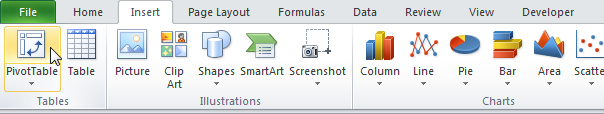
Step1: Open your Excel Spreadsheet and select values >> Go to
Insert Menu >> Click on Pivot Table.
Step2: You will see that Excel automatically selects the data for
you. Now, choose where you want the PivotTable report to be placed >>
Click OK.

Step3: Excel will now generate a new table with a blank pivot table.
Step4: The PivotTable field list appears. Now, drag the following
fields to different areas.

Step5: Below you can find the newly created pivot table.

Step6: Now you will see that how easy it is to create pivot tables, after
filtering the data.

Have a look at the two-dimensional pivot table.

Pivot Chart for the same Table:

Conclusion: As defined above that Pivot table provide great
way to summarize, examine, explore, and present your Excel file data data. So this
stepwise guide will surely help you to know how to create Pivot table in Excel.
Still you have any confusion then feel free to put a comment with your query.


Comments
Post a Comment